Jeroen Kakebeeke Sr. Investment Risk Manager at PGGM Informs on Value versus Growth stocks
Jeroen Kakebeeke is the Senior Investment Risk Manager at PGGM Investments. In this paper he reports how Quant & Fundamental analysis explain 13 years outperformance of Growth. He informs in detail the different causes for the unexpected US Growth factor outperformance versus US Value. It builds on the framework of Fama & French. Quant analysis shows changing differences in profitability for the style factors. In addition, the sensitivity of interest rate changes is calculated by a DCF model for Value and Growth factors. The interest rate causality is deducted and empirical observed. Fundamental and quant research are complementary, this leads to new insights and forecasts.
Introduction
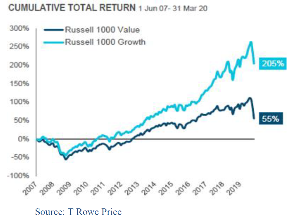
Value investing in equity is a popular way to gain outperformance. Long ago popularized by Benjamin Graham, and currently a firm building block of smart beta strategies. The idea is to reap the Value factor premium by investing in cheap companies with low valuation ratios per share (FCF, Book Value, Earnings, Sales). Academic research and asset managers have shown this approach historically has led to better returns than Growth stocks and the Market index. But not for the last 13 years!
Value Premium
The Fama & French (F&F) publication in 1992 provided global and long term evidence for the Value and Size factors. They sorted equity universes on cheapness, and ranked the 30% cheapest bucket Value, the 40% middle as Market, and the 30% most expensive bucket Growth. Value did outperform Growth, on average by 4% annually. Thus Value became a factor with a premium.There are two valid academic interpretations for Value’s outperformance. The behavioral side says that investors as a group overestimate recent profitability. The financial market is too pessimistic for Value stocks, and too optimistic for Growth stocks, whereas in reality their profitability reverts to the mean. The efficient market proponents point to a rationale in cheaper priced Value stocks. These stocks are more risky and should be compensated with higher return. More risky with cyclical revenue, leverage, more fixed assets, more competition, and a higher equity beta. Both explanations reason that Value is out of favor among investors.
Performance break down
F&F break down the Value versus Growth outperformance into a direct Dividend (1) source and three indirect sources of Capital Gain: 2a. Relative growth in book equity due to profitability (retained earnings); 2b. Converging valuation ratios due to mean reverting profitability. This is also called migration, when Value stocks promote out of the low PE bucket, and Growth vice versa; 2c. Drift in valuation ratios, or revaluation of the whole style bucket.
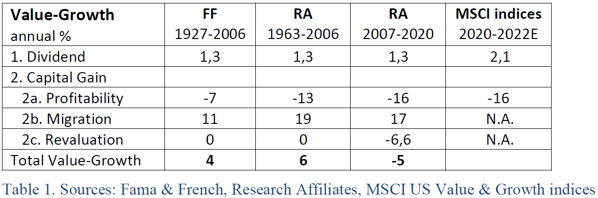
F&F updated their findings in 2006, with data starting from 1927: First, dividend was historically 1,3% higher for the Value bucket, contributing to 1/3 of the outperformance versus Growth stocks. The other 2/3 outperformance is in Capital Gain: ad 2a. Growth stocks have higher growth in book equity, a disadvantage for Value; ad 2b. The main reason of Value’s outperformance is the convergence in valuation ratios, in the PE-multiple. Annually, 20% of the Value companies migrate to ‘Market’ or Growth; ad 2c. For the Value and Growth styles, the long term PE-drift was alike.
Rare Value underperformance
The 13+ year underperformance of Value is troublesome for asset managers and painful for their clients. Asset managers point out how rare this streak of underperformance is. Based on historical data, the chance is less than 5% if you run a Monte Carlo simulation. More quant than fundamental managers do not offer any other explanation then ‘the market has become irrational’. That is unsatisfactory, I resist the idea that the market is in a bubble for so long. This mystery requires a cross examination of both a quant and fundamental view as well.
Investigation
Performance attribution helps to empirically pinpoint the four F&F sources of return, one by one. Ideally, combined with an economic explanation. The underperformance from 2007-2020 is the longest drawdown of the Value factor. To investigate these 13 years make a fine long horizon, which minimizes short term noise. Copeland et al. says: ‘Over horizons of at least 15 years, total returns to shareholders will be linked to earnings because earnings growth will track cash flow and returns to capital.’
The extreme market events of 1Q 2020 alone are unfit for a statistical analysis. Three months is ridiculously short, and especially in the Corona crisis when all parts were wildly moving. The steep drawdown of Value vs. Growth in 2017-2019 is also too short. Copeland again: ‘Changes in total returns to shareholders are linked more closely to changes in expectations than to absolute performance’. The equity market is forward looking. The stock price development has more to do with the longer term outlook, and less with quarterly reported results. On top of that, some company data in IBES or FactSet are lagging multiple months.
Quant research
Asset managers deliver data, however their results are not always comparable:
- the index used is S&P 500, Russell 1000, MSCI, or an international benchmark;
- portfolio construction is implemented by partial long-short (FF HML), some split the equity universe equally into Value versus the other half Growth, others use quartiles or deciles;
- researchers group the return-effects different than the classic F&F: Total Value Return = Dividend Income (1) + Growth in Fundamentals (2a) + Changes in Multiples (2b + 2c). Another grouping is in the structural components of Dividend (1), Operations (2a) and Migration (2b), which are persistent. Opposed to the cyclical component, Revaluation (2c).
In the end, some useful Value minus Growth figures were distilled for the US:
The structural components, have a known sign, historically and by definition:
+ dividend of the Value bucket will be larger than the dividend of the Growth bucket;
– profitability (growth in book equity from retained earnings) is much larger for Growth;
+ migration (converging PE-ratios) is always beneficial for the Value bucket.
The cyclical component revaluation is long term zero, but deviates in the short term.
The balance of these structural components was often in favor of Value stocks, but not for the last 13 years. Growth outperformance over 2007-2020 versus Value outperformance over 1963-2006 is explained by: improved Profitability of Growth over Value; less Migration of Value; and Revaluation in favor of Growth. More about these three effects below.
Profitability
Quant research from Arnott et al. (p.26) brings additional data in scope regarding profitability.
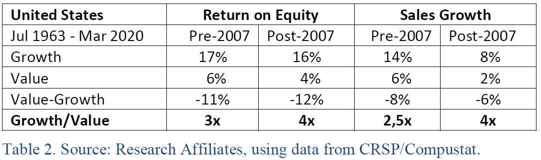
The economy over the period of 2007-2020 is characterized by secular stagnation, a lower GDP growth and lower interest rates than in the preceding decades. Regarding listed US companies, it translated into lower RoE and lower Sales Growth in buckets of Value, Market and Growth. For RoE, the absolute difference was enlarged from an 11 to 12% advantage for Growth versus Value. Growth gained from 3 times Value’s RoE pre-2007, to 4 times post-2007. For Sales Growth the factor has grown from 2,5 times pre- to 4 times post-2007.
Migration
Migration is an indirect reward of improving profitability. However, in an environment of secular stagnation Value stocks are more likely to remain Value. Post-2007, many defaults were only averted because of ultra-low interest rates by the Central Bank. Creative destruction has been delayed, some Value companies have become eternal Value, or Zombie companies.
Revaluation
Over a short horizon the PE-drift of Growth and Value buckets is driven by investor trends, or preferences. In particular the multi-year Internet hype stands out. Because eventually the market corrects, the revaluation effect is expected to be zero for the long term. However, over the last 13+ years, this effect was annually -6,6%, leading to underperformance of Value. Growth stocks benefited from better profitability (and quality) by rising investor demand (rising PE-ratio), an indirect positive revaluation. While the opposite holds for Value stocks. They are riskier in secular stagnation, and they faced falling demand (falling PE-ratio).
Revaluation was directly linked to the decline in interest rates, which is more favorable for Growth than Value. Fundamental analysis makes use of Discounted Cash Flow (DCF) modelling in pursuit of the intrinsic value of securities. This is a strong theoretical and practical model. Copeland says: ‘DCF valuations are highly sensitive to small changes in assumptions about the future. The sensitivity is also highest when interest rates are low’.
To learn about interest rate sensitivity and resulting changes in PE-multiples, I made DCF-calculations with three hypothetical stocks: Value, Market and Growth. They differ only in growth estimates of free cash flow, see the Appendix for elaboration. The DCF-results are an illustration of relative PE-multiples given the interest rate (change). They are roughly in line with observed markets. See the current MSCI US indices, and the eighties when the market-PE rose above 10 on the back of lower interest rates (and improving economic outlook).
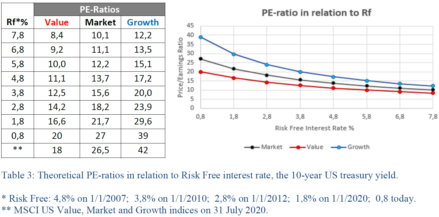
Interest rate sensitivity is clearly visible, higher PE-multiples result from lower rates, and the effect is accelerating. A new insight is how the PE-sensitivities differ in Value, Market and Growth buckets. Price returns are deducted from these revaluation effects.
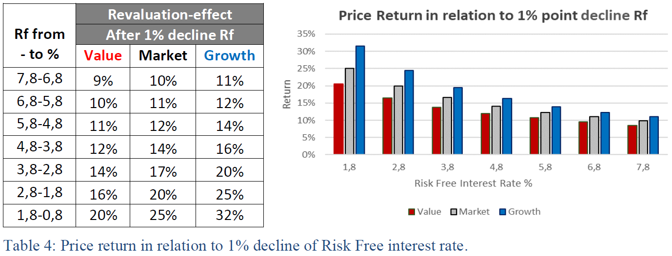
Interest rate sensitivity is visible again, and naturally accelerating with lower rates. When risk free rates decline from 7,8 to 6,8%, the theoretical price return for Market is 10%. US risk free rate declined pre- and post-Corona from 1,8 to 0,8%, lifting the theoretical PE-ratio of the market by a whopping 25% to 27x. And EPS estimates for the S&P500 index were better than anticipated, so I upgraded the price target to 3.600 in my July Investment Letter. On 15th of August, Goldman Sachs raised their S&P500 target also to 3.600, higher than other banks.
The long term causality between interest rates and equity valuation is generally known. Since 1960 lower bond yields explain lower earnings yields. Because earnings yield is the inverse of a PE-ratio, we can also say that lower bond yields explain higher PE-ratios. Never before was the sensitivity to interest rates so high, because interest rates are so low.
One could argue that the risk free interest rate is artificial low, caused by Central Bank intervention and not determined by a free market. Is it fair to calculate with such a low rate then? Yes, currently it is the observed and traded interest rate. The reality is that Central Banks will keep rates lower for longer. It is the new normal, it is part of secular stagnation. I wrote in July: ‘Central Banks will help their hefty indebted US (and European governments) with low risk free interest rates and buying government debt with new printed money. When inflation rises, debt becomes more sustainable. Thus Central Banks will not suppress inflation immediately.’ On 27th of August, Jerome Powell confirmed this idea with new inflation target.
For every interest rate the revaluation effect is stronger for Growth than Market, and less for Value than Market. This is directly linked to cash flow duration. Growth stocks’ free cash flows are further in the future, implying they have higher duration. Thus the Growth bucket benefits (much) more than the Value bucket from falling risk free interest rates. Over the period 2007 to March 2020, the risk free interest rate declined from 4,8 to 0,8%. This 4% fall has attributed annually 3,8% Growth outperformance versus Value.
And more recently, more impressive: the revaluation effect pre- and post-Corona of 1% interest rate decline, is a 12% return advantage for Growth versus Value stocks, in just a few months.
The framework of Fama & French, quant data, and the addition of the DCF interest rate sensitivities, all help to explain the outperformance of Growth. A summary of the Growth outperformance Post-2007, and the change in returns versus Value Pre-2007:
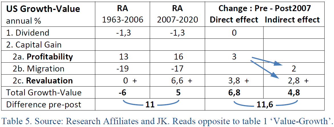
Remember, over the whole horizon US Growth underperforms by 4% annually. The pre-2007 underperformance is 6%, while that turns into 5% outperformance post-2007. The change in return of 11% annually, is explained for 3,8% by interest rate decline and the remainder by improved Profitability of Growth over Value stocks.
Japan was the first country with falling risk free interest rates nearing the zero level. Still, Value outperformed the Growth factor during the last 30 years. How come?
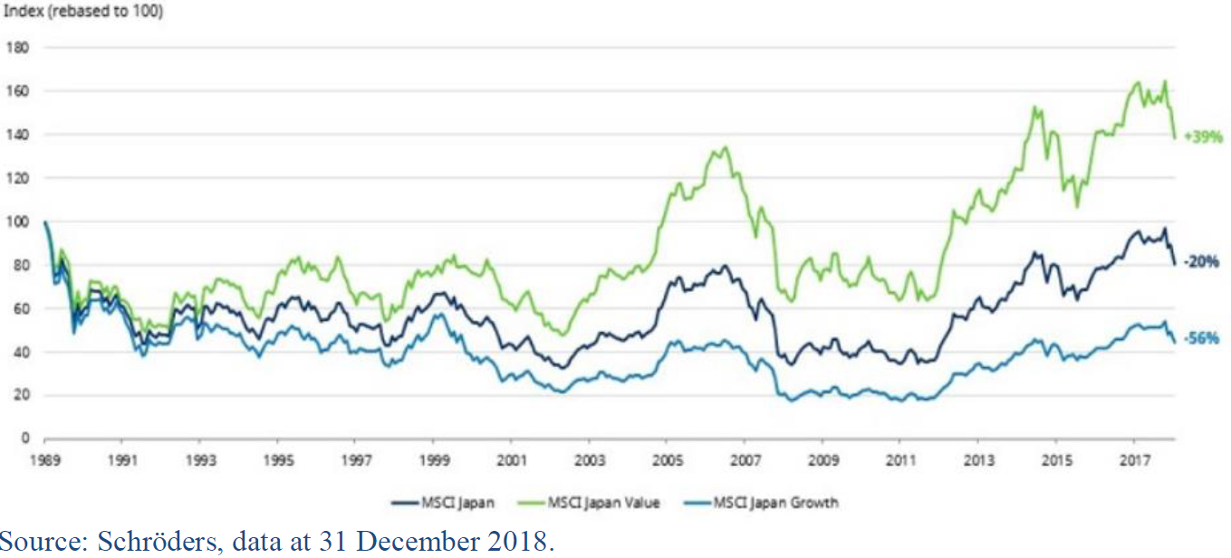
Basically, the Value outperformance versus Growth had less headwind from falling interest rates over this long horizon. Japanese Government yield declined from 5,8% to 0,8% over 30 years. From table 4, Value theoretically benefitted cumulative with 73% return, 2% annually. Growth benefitted cumulative with 107%, annually 2,7%. The disadvantage of Japanese Value is only 0,7% annually, whereas US Value had a disadvantage of 3,8% annually. So, the Japanese decline in risk free interest rates had a minor effect.
Conclusions
1. Quant and fundamental research are complementary and this leads to new insights.
2. The outperformance of Growth versus Value over the last 13+ year is attributable to:
- improved profitability of Growth stocks over Value stocks; and
- Growth stocks benefitted most from the decline in risk free interest rates.
Thesis
The idea of mean reversion is attractive, however, for Value to outperform Growth it is important that risk free interest rates do not decline further.
Other views on the role of interest rates in Growth versus Value
BMO’s Head of Strategy spoke briefly about the underperformance of the Value Factor on 28 May 2020: ‘First of all, it is about the interest rate. In a Discounted Cash Flow model, the interest rate is the factor to settle a future cash flow to the present. Value has mainly its cash flows now, whereas Growth has its cash flows further away. So a decline in interest rates has driven the outperformance of Growth, and we probably need to see an upward move in interest rates for Value to outperform.’
Henry Dixon, Man GLG on 30 July 2020: ‘The headwind of falling bond yields to Value has been almost entirely one way over the past decade. In the Taper Tantrum of 2013 we saw interest rate rises. Consequently, the Diageo PE-ratio (Growth stock) declined by 15%, the Aviva PE-ratio (Value stock) increased by 15%. These examples paint a picture for a general Growth-Value performance attribution. Rising interest rates are not a necessary catalyst, but will for sure help the Value style.’
Strategist Katie Trowsdale at Aberdeen recommends that investors start looking at Value again when Corona is away. The economy can recover, including inflation, and the monetary policy will normalize. This leads to higher interest rates, and Value can regain performance.
Scott Berg is the portfolio manager for the T. Rowe Price Global Growth Equity Strategy, and wrote in August 2020: ‘A final caveat on valuations is that we are clearly now in a world where interest rates are going to be lower for even longer than we previously thought, perhaps much longer. The dividend discount model, other things equal, suggests that in a world where the risk‑free rate is expected to be much lower, there is a respectable argument that equity valuations can be meaningfully higher.’
Those four fundamental views happened to pass by. These views support the effect interest rate declines had on Growth’s outperformance, and the outlook for Value’s outperformance.
AQR’s Maloney and Moskowitz (M&M) received attention with their paper from May 2020. They perform statistical analysis on equity returns and interest rates. M&M conclude that the performance of Value is not easily assessed based on the interest rate environment: ‘Empirically, we find fairly modest links. Evidence of a mild relationship between interest rate variables and Value’s performance is found for some specifications, but not others. Despite some eye-catching patterns in recent data, particularly those related to changes in bond yields or the yield curve slope, the economic significance of any relationship is small and not robust in other samples.’
In my opinion, their method is too straightforward with only one explanatory variable. Thus less applicable in a complex debate of Value versus Growth. M&M emphasize that in the real world an interest rate change is never ceteris paribus. They enumerate (un)expected changes in cash flows, economic growth, inflation, the equity risk premium. Unfortunately, further research on these changes is absent. It could be an idea for a follow up paper.
In the framework of F&F, interest rate (change) has only an effect on the Residual component. M&M neglect the three components Dividends, Profitability and Migration, which are larger and volatile. As a comparison, their method would calculate the effect wind has on the speed of a sailing boat. Taking into account the wind’s force and direction. But not correcting for the number of sails, the hull speed, nor the current from low and high tide. Also, their conclusion could be more specific. When the interest rate is low, there is a significant and economic meaning full correlation in a change of interest rate!
US Value Factor sensitivity to US 10-year yield changes 1954-2019 (rolling 10-year t-stat)
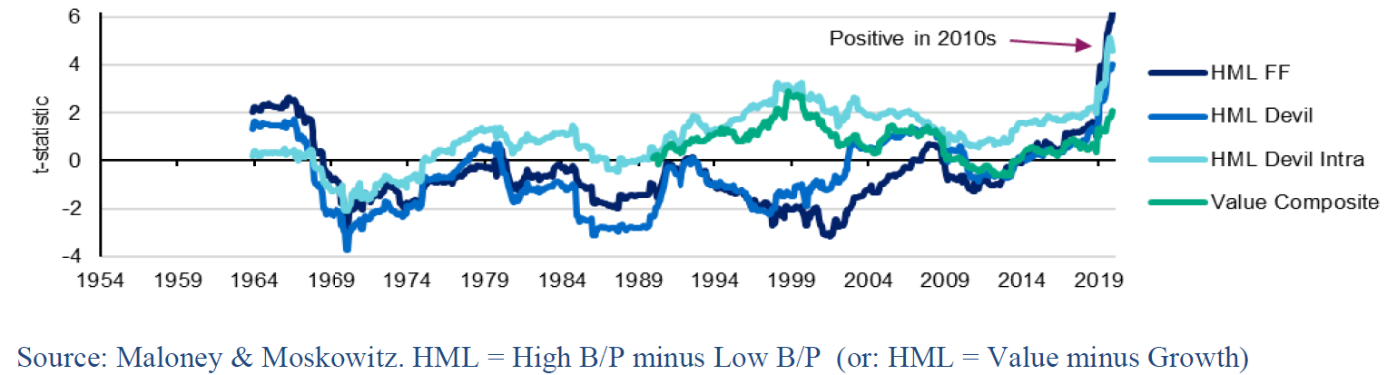
At least, Maloney and Moskowitz confirm in their graph strong causality of interest rates on Value-minus-Growth buckets, in line with the DCF model and my conclusion. When the risk free interest rate declined sharply over the period 2007-2019, to the lowest level ever, the t-statistics jumps significantly.
Outlook for the Value Factor
The US Growth bucket is on average 5,4 times as expensive as the Value bucket, based on Price/Book. In the eighties, with high interest rates, high inflation, weak economic growth, the ratio was lowest at 4. Also remarkably, the ratio was low at the end of 2006. Value seemed expensive and/or Growth cheap, a fine starting position for a Growth outperformance. Today, with low interest rate, low inflation, and decent profit growth, the ratio is highest at 10 times.
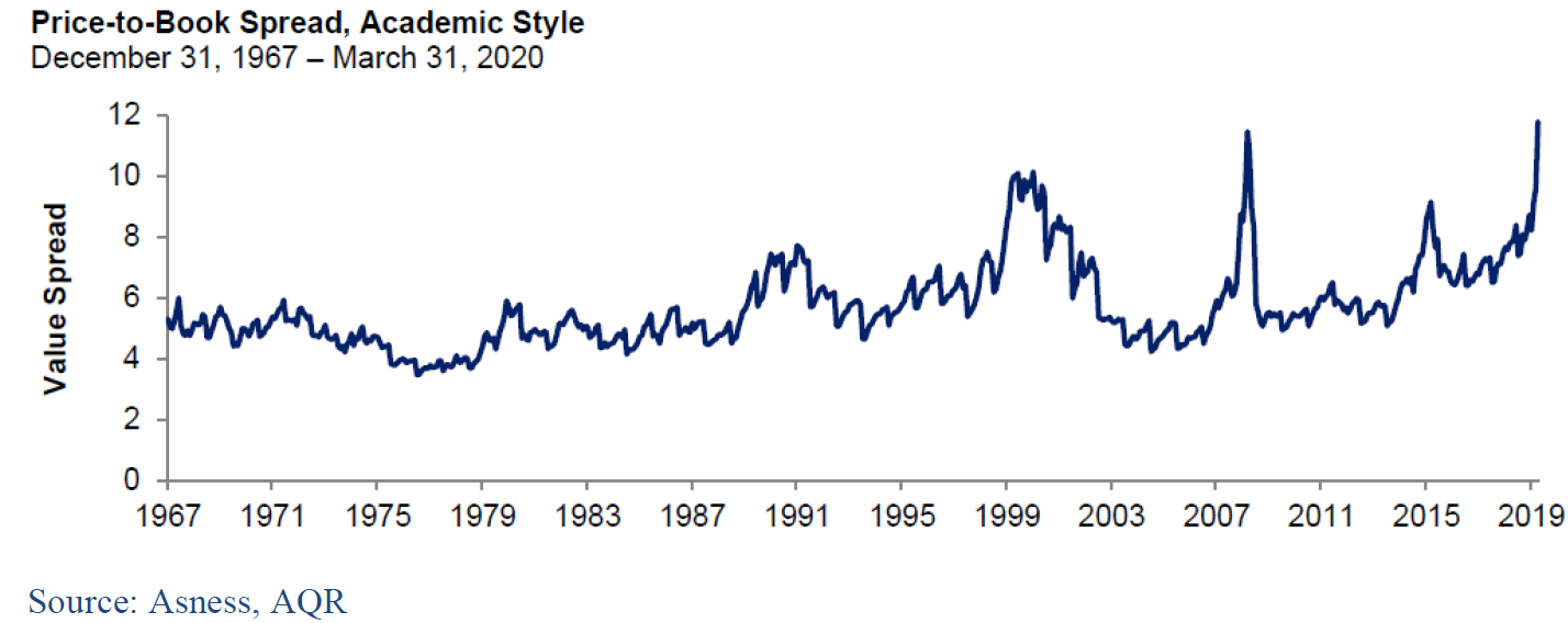
Realize the value spread will come down automatically, when new estimates are fed into the consensus systems. ‘Price’ has immediately adapted in the COVID-19 crisis, whereas ‘Book Value’ is a lagging indicator. The Growth bucket will increase its Book Value, Sales, Earnings. FAMAG are Labor Light and Asset Light, no machinery, factories, or inventories. So they are very flexible to adapt, what especially in a crisis, is a big advantage. The Value bucket can only report declines, driven by the sectors Energy, Financials, Real Estate. And by industries like Automobile, Airline and Hotels. However, the ratio remains probably elevated, pointing to an attractive entry point for Value. Even after correcting for incomplete treatment of ‘intangibles’, assets that are not physical in nature and that are hard to define or measure.
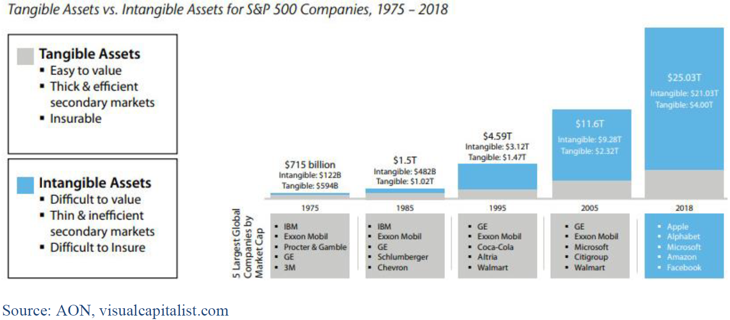
Intangibles
The traditional Book/Price ratio has difficulties in capturing real asset growth since intangibles become much more important. In just 43 years, intangibles have evolved from a supporting asset into a major consideration for investors. Last year, they made up 84% of all enterprise value on the S&P 500, a massive increase from just 17% in 1975. Especially the FAMAG shares stand out: Facebook, Amazon, Microsoft, Apple and Google.
Investors agree that more transparency would be beneficial to their assessment of intangible assets. In the absence of robust reporting, Columbia Threadneedle believes active managers are well equipped to understand intangible asset values due to their access to management, relationships with key opinion leaders, and deep industry expertise.
Arnott cum suis from Research Affiliates explore whether value is mis-measured when using book value, given current US accounting standards that ignore internally created intangible investments. The authors find that a measure of value calculated with capitalized intangibles (iHML) outperforms the traditional B/P measure for the period beginning in the 1990s, which coincides with the internet revolution and the importance of intangible assets.
Second thesis
I am an optimist: we can restrain COVID-19, we will develop our economies in a sustainable way. Say 2% GDP growth and 2% inflation longer term. A risk free debtor like the US government has to compensate investors only for inflation. Consequently, US 10-year interest rates will slowly rise to 2%. Together with decent company profits, I see value in Value. Growth will not tumble, but the estimates for Value-minus-Growth are too negative.
drs Jeroen Kakebeeke RBA is an Advisory Board member of Institutional Investor working as Investment Risk Manager for a large pension fund. The views expressed in this paper are his own. The author thanks Kiemthin Tjong Tjin Joe for his valuable ideas. To discuss the content of this article and further engage with him, comment below or Sign up today.
References
Arnott, R.C., 2020, Reports of value’s death may be greatly exaggerated. Research Affiliates
Asness. C., May 2020, Is (Systematic) Value Investing Dead? AQR
Copeland, T., et al., 2000, Measuring and managing the value of companies. Wiley
Fama, E.F. & K.R. French, 2007, The Anatomy of Value and Growth Stock Returns. Financial Analysts Journal, Volume 63, Issue 6, p. 44-54.
Ilmanen, A., 2011, Expected returns. An investor’s guide to harvesting market rewards. Wiley
Maloney T. and T. J. Moskowitz, May 2020, Value and Interest Rates: Are Rates to Blame for Value’s Torments? AQR
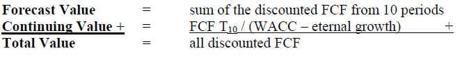
Appendix: DCF-model
To calculate the discounted cash flow of three hypothetical stocks Value, Market and Growth. The only difference is the growth rate of Free Cash Flow (j, k).
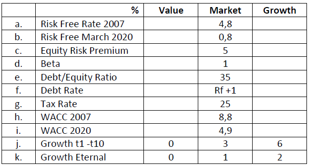
The Risk Free interest rate is approximated by the 10 year US-treasury, as recommended by Copeland and other researchers.
b. Over the period 2007 to March 2020 the Risk Free interest rate declined by 4%.
c. Copeland et al. ‘recommend a 4,5% to 5% premium for the US market’. With a 4% ERP suggested by Ilmanen (p.125), the interest rate effects are larger.
d. Beta of 1 (by definition).
e. For the Debt/Equity Ratio Russell measured an average of 35% for the US.
f. The credit spread is fixed at 1% above Risk Free.
g. Effective US corporate tax was on average 25%.
h. In 2007 the Weighted Average Cost of Capital was 8,8%.
i. Over the period 2007-2020 the WACC declined by 3,9% to 4,9% for all stocks.
j. The explicit forecast has a duration of 10 periods. The estimated growth is 0% for Value, 3% for Market and 6% for Growth. The growth difference narrows in the eternal forecast. Because of competition, growth come down over longer horizons. Market growth falls to 1%, equal to GDP in a lower for longer scenario.
For one unit of Free Cash Flow (FCF), the model calculates intrinsic value as follows: